The statistic at the core of Fastly’s capacity model usually appears in economics papers. The Gini coefficient is a macroeconomic metric used to describe inequality in a population. Fastly's capacity questions are seemingly much more concrete. We need to know whether a POP can handle a major game release, how much headroom exists across a continent for a live sporting event, what happens as AI and security workloads continue their rapid growth, and where we should invest in infrastructure months or years into the future.

But it turned out the Gini coefficient was the key to our capacity planning.

Major events change the shape of the traffic we serve. A normal day at Fastly involves massive diversity of customer workloads, service changes, and object popularity shifts. During a major game release, software update, live event, or shift away from another provider, a small number of workloads can suddenly account for a large fraction of traffic.

This observation became the core of the capacity model that Fastly uses today:

traffic inequality -> cache behavior -> CPU utilization -> headroom

The surprise was how much this one signal explained. I first tried a long list of machine learning and forecasting approaches: AutoML systems, neural nets, tree models, ensembles, regressions, specialized time-series prediction models, and even LLMs. Many worked well on ordinary traffic, but they struggled with the rare cases that matter most for capacity planning.

The model that won is small, interpretable, and fast enough for interactive scenario analysis. It has now been in production use for more than a year.

The key was treating traffic inequality as a first-class signal.

Capacity at the Edge is a Workload Question

A Fastly POP does not have one simple number called capacity. Fastly POPs consist of bare-metal servers running a mixed workload on Fastly's intricate and high-performance software stack. The traffic mix varies by region, customer, time of day, and event. POPs have live video, API traffic, security workloads, software downloads, mixed web traffic, and wasm-based Compute workloads all at the same time. Each additional request, Gbps of traffic, or compute task can be wildly different depending on what it is. POPs are built over time, so the hardware mix also reflects when and where the infrastructure was deployed.

That makes planning a practical systems problem rather than a clean or abstract resource-allocation problem. A POP with plenty of headroom on one day might be gasping for air on a different day even if the workloads look superficially similar.

We need to be able to plan for the common case and handle the uncommon case. That means we ask questions like these:

• Can this POP carry a known event next week?

• How much additional bulk-download traffic can this region absorb?

• What if Compute and Security grows twice as fast as delivery traffic?

• Which group of processes becomes CPU limiting first?

• How much headroom remains above normal seasonal traffic?

• Where should we build more capacity?

• What happens when customer traffic moves to Fastly during a failover away from another provider?

Traffic can shift to Fastly for many reasons: customer routing decisions, planned events, traffic migrations, maintenance, or incidents elsewhere in the internet. The capacity model needs to handle those shifts as ordinary planning scenarios.

A useful model has to support counterfactuals. We don't often try to predict what will happen next, because we expect the unexpected. We care more about what would happen in a variety of scenarios.

Off-the-shelf AI and ML Was Not Enough

At first this looked like a conventional AI / ML problem. We have so much telemetry that it's like a kid in a candy store for AI / ML: thousands of metrics about traffic, request rates, compute tasks, internet weather, cache behavior, CPU utilization, and so much more. It was natural to try the standard toolbox of AI and ML techniques available in popular open-source packages and various vendors' proprietary offerings.

Many of these standard techniques produced good average case error. They learned normal traffic well, so on ordinary days the predictions could look quite good. However, capacity planning is defined by its unusual days.

The generic models often learned broad relationships like:

more bytes -> more CPU
more requests -> more CPU
more wasm compute -> more CPU

Which is what they should have learned from the data. The problem is the strength of those relationships varies depending on the particulars of the workload, and those particulars weren't picked up by any of the generic models, no matter how sophisticated they were.

An edge version of inequality

The Gini coefficient measures inequality across a set of values such as incomes. But in our edge infrastructure, the key inequality is between customer workloads: the shape of traffic that is dominant at a specific time.

The key observation is that our algorithms are implicitly tuned for cases where one type of traffic is dominant. Caching, at every layer from the processor to the POP, benefits from popularity. A cache makes serving hot data less computationally intensive than fetching and providing cold data from somewhere else. It turns out that popularity is just a form of inequality, and the Gini coefficient is the right metric for measuring that inequality. It gave us a number for that popularity signal without requiring the model to know the name of the game, the event, the customer, or the launch schedule.

The clearest place where this shows up is the cache hit ratio. A diffuse workload might have thousands of customers contributing small shares of traffic. A major release or live event might have a couple of customers accounting for most of the traffic in a POP. Those two cases can have the same total traffic volume and very different cache behavior: I found traffic inequality in the form of the Gini coefficient, once rescaled, tracked edge cache behavior during the most extreme circumstances that we often were planning around. It also turned out that those events were exactly the same ones that generic AI and ML techniques performed the worst on, because they were extreme, unpredictable outliers.

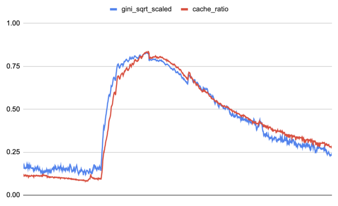
The rescaled square root of the Gini coefficient versus the front-end cache hit ratio at our EWR POP before, during, and after a major game release.

That observation led to a cache model separate from POP CPU utilization:

gini = Gini coefficient over the top customer traffic fractions

top_N_ratio = fraction of traffic from the N largest customers

predicted_cache_hit_ratio = a * sqrt(gini)
                          + b * top_N_ratio
                          + c

The coefficients in this come from robust regression over recent history. Including the top N customers, in addition to the Gini coefficient, captures a similar intuition and matters for POPs where the traffic is notably less diverse. The prediction is clipped to a reasonable range. We also use our telemetry to account for customers whose traffic is structurally less cacheable, so that concentration of an uncacheable workload does not get mistaken for useful cache locality.

The square root was a small but important rescaling. Cache behavior did not appear to improve linearly with traffic inequality. The first signs of concentration mattered a lot: they meant traffic was becoming popular enough for the cache to exploit. After traffic was already highly concentrated, additional inequality had diminishing returns. Taking the square root stretched the low and middle range of the Gini coefficient and compressed the high end, aligning the two.

Incorporating inequality into CPU utilization

Let's return to CPU utilization. The first models I built, using various standard AI/ML techniques, were meant to predict CPU utilization from traffic:

traffic mix -> predicted CPU -> POP capacity/headroom

Once you know the predicted CPU, you can run scenarios with different traffic mixes and see what CPU levels you hit. Simulating higher and higher traffic volumes will get you to a CPU ceiling, which tells you the POP's capacity and headroom.

With cache behavior as the key to unlocking accurate modeling of POP capacity, complex AI/ML techniques turned out to no longer be necessary. The production model is now remarkably simple.

First, it predicts the front-end cache hit ratio from traffic concentration using the approach above. The front-end cache hit ratio is key to CPU efficiency because it tells us whether an object can be served without asking the cluster primary, whereas the cluster and POP-wide cache hit ratios (which are much higher) tell us more about origin offload.

Second, it predicts CPU from traffic, request rate, compute task volume, and the cache prediction as follows:

traffic mix -> predicted cache ratio -> predicted CPU -> POP capacity/headroom
            |                        |
            --------------------------

We train per POP. The models are trained separately for the relevant CPU groups on our servers. The features of this model are intentionally narrow and operational:

bits per second
requests per second
compute task volume

The CPU utilization model uses robust regression on these features at 1 minute granularity. We filter out low-CPU rows before fitting, because very quiet periods are less informative for capacity planning. We also overweight high-CPU samples when fitting the cache multiplier, because the upper range is where planning decisions happen.

During training we use real front-end cache hit ratio data and during inference we first run the Gini-based cache hit ratio model and feed its output forward. For a hypothetical event, we do not know the cache hit ratio. The model has to predict the cache behavior that traffic mix would create, then predict the CPU that would follow. The cache multiplier captures the way better cache behavior reduces CPU cost, with cutoff and power constants determined through a simple grid search:

downshifted = max(cache_hit_ratio - cutoff, 0)

multiplier = 1 - downshifted ^ power

predicted_cpu_utilization = base_cpu_utilization * multiplier

This model has near-instant inference. Planners and engineers can vary the POP, baseline, customer, workload type, and growth scenario rapidly. The output also has useful intermediate values: traffic concentration, predicted cache ratio, cache multiplier, base CPU prediction, final CPU prediction, and limiting CPU group. The model's simplicity aids in its interpretability.

Despite the wide range of traffic shapes that Fastly encounters in the wild, we find that this simple model keeps within 5% of real CPU utilization whereas more sophisticated models would often deviate by 25% or more.

Headroom Depends on the Scenario

A POP can have one amount of headroom for uniform growth, another for compute-heavy growth, another for a bulk download, and another for a live event. The model has to make those assumptions visible.

The headroom loop starts from a representative baseline. Then it scales traffic according to a scenario and runs the prediction chain until a CPU threshold is reached.

choose a scenario and baseline timestamp

use binary search to find traffic level just below CPU groups max threshold:
  predict cache behavior for the scaled traffic mix
  predict CPU from traffic, compute volume, and predicted cache behavior

The output includes the limiting CPU group, predicted CPU at the limit, additional Gbps or RPS, Compute task headroom where relevant, and per-server capacity. The final planning answer also considers network constraints such as NIC, peering, and transit capacity.

This framing has been useful for event planning because it lets us ask the same question many ways. A planner can compare a near-peak baseline with an off-peak baseline, a uniform-growth assumption with a customer-specific bulk event, or a delivery-heavy customer ramp with a compute-heavy one.

Finding a Normal Baseline

We need a baseline that represents normal traffic for a POP. A baseline should avoid unknown events, outages, or unexpected traffic behavior. Otherwise, the headroom calculation starts from an uninterpretable baseline.

As with the CPU model, I expected sophisticated models for time-series prediction to help here, but once again they didn't. For this use case, the best approach was seasonal naive forecasting from statsforecast.

Seasonal naive forecasting is plain: recent seasonal behavior predicts normal future behavior. Internet traffic has strong daily and weekly rhythms, so this simple method gave us a reliable way to identify ordinary days. More flexible systems, including Prophet-style models, were often less useful for selecting normal baselines. They introduced complexity that did not improve the planning decision.

This reinforced the broader lesson from the CPU model. The best model was the one that matched the operational question.

From Prediction to Placement

Once we could see traffic concentration as a cache-efficiency signal, we could reason about placement differently. Spreading traffic evenly is a natural instinct in distributed systems. But for some edge workloads, deliberate concentration can improve efficiency and performance because it increases cache locality.

That does not mean every workload should be concentrated. Concentration has limits and risks. It can create hot spots, reduce failure isolation, or push a POP toward another constraint. The model gives us a way to evaluate those tradeoffs quantitatively.

For compatible workloads, we have used the inequality insight to concentrate traffic intentionally and improve efficiency, especially on older hardware. The same hardware can behave differently depending on whether it is serving diffuse long-tail traffic or popular cache-friendly traffic. A model that understands traffic concentration lets us find those opportunities without guessing.

This is one of the more interesting outcomes of this model. It started as a way to predict POP headroom and led to us changing certain traffic shapes to maximize efficiency.

Simplicity and Production Use

This model has been in production at Fastly for more than a year. We've used it to understand our capacity for major game releases, for POP builds around the world, and more.

The final model is simple because the problem structure is explicit. A more complex model can sometimes infer hidden relationships from enough data. Our most important cases were intermittent, heterogeneous, and operationally sensitive. It didn't make sense to hope for a generic model to infer the right structure from intermittent events.

The cache model is a robust regression over Gini and top-customer concentration. The CPU model is a robust regression with a cache multiplier and high-CPU weighting. The headroom analysis is a search over scaled traffic scenarios.

The lesson I took from this is that feature engineering still matters when the features capture the underlying system behavior. The Gini coefficient worked because it described something real about edge traffic. It converted a vague operational intuition that popular things cache well into a measurable input the model could use.

That's why a macroeconomic metric ended up in Fastly's capacity model, and why the model became more powerful when it became simpler.